Physics of Bouncing Balls: How a Bouncing Ball Works
Explore the physics of a bouncing ball: from kinematic equations to energy dissipation. Learn about gravity, restitution, and Newton's laws with our interactive JS simulator.
Phase 1: Observation and Basic Kinematics (Introductory Level)
To a beginner, a bouncing ball serves as a perfect introduction to Kinematics—the branch of mechanics concerned with the motion of objects without reference to the forces which cause the motion. In this stage, we focus on tracking state changes over time using two primary vectors: Position ($\vec{s}$) and Velocity ($\vec{v}$).
Understanding Motion: The Language of Physics
Before we can understand a bouncing ball, we must establish a vocabulary. In physics, we describe motion using several fundamental quantities. Position tells us where an object is located in space, typically measured from a reference point called the origin. Displacement describes the change in position—not the path traveled, but the straight-line distance from start to finish. Velocity measures how quickly position changes, combining both speed and direction. Finally, Acceleration describes how velocity itself changes over time.
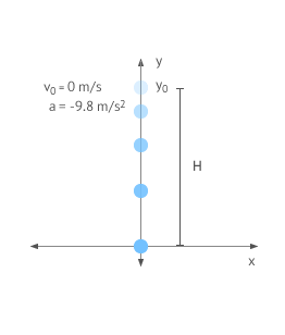
Consider dropping a ball from your hand. At the moment of release, its position is at hand height, its velocity is zero (it hasn't started moving yet), but its acceleration is already $9.81 m/s^2$ downward due to gravity. This seemingly simple scenario already involves all the fundamental kinematic quantities working together.
The Coordinate System: Choosing Your Frame of Reference
In computer graphics and physics simulations, we typically use a Cartesian coordinate system. The origin (0,0) is usually placed at the top-left corner of the screen, with the x-axis extending rightward and the y-axis extending downward. This differs from traditional mathematics, where y increases upward. Understanding your coordinate system is crucial—a positive velocity in the y-direction means downward motion in most programming environments.
The Geometry of the 'Bounce'
In an idealized world of Uniform Linear Motion (ULM), we assume the ball moves at a constant speed. The 'Physics' here is purely geometric and conditional. We define a boundary (the floor) and monitor the ball's coordinates. When a coordinate exceeds that boundary, we trigger a 'Reflection Event.'
- Independence of Axes: We treat $x$ (horizontal) and $y$ (vertical) motion separately. Unless an external force acts horizontally, the ball continues its sideways journey at a constant rate. This principle, known as the Independence of Perpendicular Motions, was first clearly articulated by Galileo and forms the foundation of projectile motion analysis.
- Velocity Inversion: The moment of impact is modeled by multiplying the vertical velocity by $-1$. This represents a perfect, instantaneous change in direction. While physically unrealistic (real collisions take finite time), this approximation works well when the collision duration is much shorter than the time between simulation frames.
- The Overlap Problem: In digital frames, a ball might move 'into' the floor between two frames. We must perform a Positional Correction (or 'teleportation') to reset the ball exactly at the boundary surface to prevent visual glitching or 'sticking'. This is one of the fundamental challenges in discrete-time simulation.
Time Discretization: From Continuous to Frame-Based
Real physics operates continuously—a ball's position changes smoothly through every infinitesimal moment. Computer simulations, however, must approximate this continuity using discrete time steps, often called frames or ticks. If your game runs at 60 frames per second, physics updates occur every $1/60 \approx 0.0167$ seconds. This fundamental constraint shapes how we implement physics algorithms.
The choice of time step ($\Delta t$) creates a tradeoff. Smaller time steps yield more accurate simulations but require more computational power. Larger time steps are faster but can miss collisions or produce unstable behavior. Most game engines use fixed time steps (constant $\Delta t$) for physics while allowing variable frame rates for rendering, preventing physics from becoming frame-rate dependent.
// Simple Position Update (Uniform Motion)
class SimpleBall {
  constructor(x, y, vx, vy) {
    this.x = x;    // Current x position
    this.y = y;    // Current y position
    this.vx = vx;  // Velocity in x direction (constant)
    this.vy = vy;  // Velocity in y direction (constant)
  }

  update(deltaTime) {
    // Displacement = velocity × time
    // In the simplest case, just add velocity to position
    this.x += this.vx * deltaTime;
    this.y += this.vy * deltaTime;
  }

  checkFloorCollision(floorY) {
    if (this.y >= floorY) {
      // Positional correction: move ball back to floor surface
      this.y = floorY;

      // Velocity inversion: perfect elastic collision
      this.vy = -this.vy;
    }
  }
}

// Usage example:
const ball = new SimpleBall(100, 50, 5, 3);
const timestep = 1/60; // 60 FPS

function gameLoop() {
  ball.update(timestep);
  ball.checkFloorCollision(400); // Floor at y=400
  // ... rendering code ...
}Phase 1.5: Introducing Motion Graphs (Bridge Level)
Before we add forces and acceleration, let's develop our intuition by visualizing motion through graphs. Motion graphs are powerful tools that translate abstract equations into visual patterns, helping us predict and understand an object's behavior.
The Position-Time Graph
For uniform motion, a position-time graph is a straight line. The slope of this line equals the velocity. A steeper slope means faster motion. A horizontal line means the object is stationary ($v = 0$). A negative slope indicates motion in the negative direction. For a ball bouncing with constant velocity (our Phase 1 model), we'd see a zigzag pattern—straight lines with slope $+v$ going down, then slope $-v$ going up, creating a sawtooth wave.
The Velocity-Time Graph
In the constant velocity model, the velocity-time graph shows horizontal lines that instantly flip from positive to negative at each bounce. These instantaneous jumps are physically impossible (infinite acceleration!) but serve as a useful approximation. The area under a velocity-time curve represents displacement—a fundamental relationship we'll use extensively in more advanced analysis.
Predicting Behavior from Graphs
Let's practice graph reading with a thought experiment. Imagine a velocity-time graph showing a horizontal line at $v = 5 m/s$ for 3 seconds, then a horizontal line at $v = -3 m/s$ for 2 seconds. Without calculation, we know the object moved 15 meters in the positive direction (area = $5 \times 3$), then 6 meters in the negative direction (area = $3 \times 2$), for a net displacement of 9 meters positive. This 'area interpretation' becomes crucial when dealing with changing velocities.
Phase 2: Dynamics and Constant Acceleration (Intermediate Level)
Moving beyond simple motion, we introduce Dynamics—the study of forces and their effects on motion. Real objects are governed by Newton's Second Law ($\vec{F} = m\vec{a}$), where forces cause changes in velocity. On Earth, the dominant force is Gravity ($F_g = mg$), which exerts a constant downward pull.
Newton's Laws: The Foundation of Classical Mechanics
Sir Isaac Newton's three laws form the cornerstone of classical physics. The First Law (Law of Inertia) states that an object maintains its velocity unless acted upon by a net force. The Second Law quantifies this: the acceleration of an object is directly proportional to the net force and inversely proportional to its mass ($a = F/m$). The Third Law reminds us that forces come in pairs: for every action, there's an equal and opposite reaction.
For our bouncing ball, gravity provides a constant downward force of $F_g = mg$. Since the mass is constant, this produces a constant downward acceleration of $a = g \approx 9.81 m/s^2$. This seemingly simple scenario contains profound implications: velocity no longer remains constant but changes linearly with time, and position no longer changes linearly but follows a quadratic curve.
The Quadratic Path: Understanding Parabolas
Because gravity provides a constant acceleration ($g \approx 9.81 m/s^2$), the velocity is no longer constant—it increases linearly over time. Consequently, the position changes quadratically. This is the origin of the parabolic arc seen in every sports game or animation.
The complete kinematic equations for constant acceleration are known as the SUVAT equations (named after the variables: displacement, initial velocity, final velocity, acceleration, and time). These equations allow us to solve for any unknown given sufficient information about the others:
For a bouncing ball where $a = g$ and we're measuring vertical position:
This equation allows us to predict exactly where the ball will be at any given second. In a simulation, however, we usually calculate this incrementally, frame by frame, adding a small 'slice' of gravity to the velocity in every update.

Deriving the Kinematic Equations
Understanding where these equations come from deepens your physical intuition. Starting with the definition of acceleration as the rate of change of velocity: $a = \frac{dv}{dt}$. For constant acceleration, we can rearrange and integrate: $dv = a \, dt$, which gives us $\int_{v_0}^{v} dv = \int_{0}^{t} a \, dt$. Since $a$ is constant, this yields $v - v_0 = at$, or $v = v_0 + at$.
Now, knowing that velocity is the rate of change of position ($v = \frac{ds}{dt}$), we can substitute our velocity equation: $\frac{ds}{dt} = v_0 + at$. Integrating again: $\int_{s_0}^{s} ds = \int_{0}^{t} (v_0 + at) \, dt$. This yields $s - s_0 = v_0 t + \frac{1}{2}at^2$, giving us the position equation. This calculus-based derivation reveals that these equations are not arbitrary formulas but fundamental consequences of constant acceleration.
Projectile Motion: Combining Horizontal and Vertical
When a ball bounces at an angle, we see the full beauty of projectile motion. The horizontal motion (in the absence of air resistance) follows uniform motion: $x(t) = x_0 + v_{0x}t$. The vertical motion follows accelerated motion: $y(t) = y_0 + v_{0y}t + \frac{1}{2}gt^2$. These two independent motions combine to create the characteristic parabolic trajectory.
We can eliminate time from these equations to find the path equation directly. From the horizontal equation: $t = \frac{x - x_0}{v_{0x}}$. Substituting into the vertical equation yields: $y = y_0 + v_{0y}\frac{(x-x_0)}{v_{0x}} + \frac{1}{2}g\left(\frac{x-x_0}{v_{0x}}\right)^2$. This is a quadratic equation in $x$, confirming the parabolic shape mathematically.
// Implementing Constant Acceleration (Gravity)
class AcceleratedBall {
  constructor(x, y, vx, vy, radius) {
    this.x = x;
    this.y = y;
    this.vx = vx;
    this.vy = vy;
    this.radius = radius;
  }

  update(deltaTime, gravity = 9.81) {
    // DYNAMICS: Apply gravitational acceleration
    // Using Semi-Implicit Euler (velocity first, then position)
    this.vy += gravity * deltaTime;

    // KINEMATICS: Update position based on new velocity
    this.x += this.vx * deltaTime;
    this.y += this.vy * deltaTime;
  }

  checkFloorCollision(floorY, restitution = 1.0) {
    if (this.y + this.radius >= floorY) {
      // Positional correction
      this.y = floorY - this.radius;

      // Velocity reversal with energy loss
      this.vy *= -restitution;

      // Prevent micro-bouncing
      if (Math.abs(this.vy) < 0.5) {
        this.vy = 0;
      }
    }
  }
}

// Comparison: Explicit vs Semi-Implicit Euler
class ExplicitEulerBall {
  update(deltaTime, gravity) {
    // EXPLICIT: Update position first using OLD velocity
    this.x += this.vx * deltaTime;
    this.y += this.vy * deltaTime;

    // Then update velocity
    this.vy += gravity * deltaTime;
    // Less stable, tends to gain energy over time!
  }
}

class SemiImplicitEulerBall {
  update(deltaTime, gravity) {
    // SEMI-IMPLICIT: Update velocity first
    this.vy += gravity * deltaTime;

    // Then update position using NEW velocity
    this.x += this.vx * deltaTime;
    this.y += this.vy * deltaTime;
    // More stable, conserves energy better!
  }
}Phase 2.5: Forces and Force Diagrams (Intermediate-Advanced Bridge)
To truly understand dynamics, we must think in terms of forces. Every change in motion—every acceleration—has a force behind it. Learning to identify, diagram, and analyze forces is essential for solving complex physics problems.
Free Body Diagrams: Isolating the Object
A Free Body Diagram (FBD) is a simplified sketch showing an object as a point or simple shape with all forces acting on it drawn as arrows. The length of each arrow represents the magnitude of the force, and the direction shows which way the force acts. For a ball in mid-air, the FBD shows only one force: gravity pulling downward with magnitude $mg$.
When the ball contacts the floor, our FBD becomes more complex. Now we have two forces: gravity $F_g$ downward and the normal force $F_N$ upward from the floor. The normal force is perpendicular to the contact surface (hence 'normal'—a term borrowed from geometry meaning perpendicular). During the brief collision, $F_N$ vastly exceeds $F_g$, creating a large net upward force that rapidly decelerates the ball, brings it momentarily to rest, then accelerates it upward again.
Multiple Forces: Vector Addition
When multiple forces act on an object, we must find the net force (or resultant force) by vector addition. Forces are vectors—they have both magnitude and direction—so simple arithmetic doesn't work. We must add them using the parallelogram rule or by adding components. For forces aligned with coordinate axes, component addition is straightforward: $F_{net,x} = \sum F_x$ and $F_{net,y} = \sum F_y$.
Consider a ball rolling on a surface with friction. We have gravity $F_g$ downward, normal force $F_N$ upward (these cancel in the vertical direction if the surface is level), and friction $F_f$ opposing the motion horizontally. The net force is purely horizontal: $F_{net} = -F_f$, causing the ball to decelerate. This demonstrates an important principle: forces in perpendicular directions can be analyzed independently.
Contact Forces vs Field Forces
Forces fall into two broad categories. Contact forces require physical touching—examples include normal force, friction, tension in a rope, and air resistance. Field forces act at a distance through space—gravity, electric force, and magnetic force. In our bouncing ball, gravity is a field force acting continuously throughout the ball's flight, while the normal force is a contact force acting only during the brief collision with the floor.
Impulse and Momentum: Alternative Perspectives
While $\vec{F} = m\vec{a}$ is the most common form of Newton's Second Law, an alternative formulation uses momentum ($\vec{p} = m\vec{v}$): $\vec{F} = \frac{d\vec{p}}{dt}$. This states that force equals the rate of change of momentum. Integrating both sides over a time interval gives us the Impulse-Momentum Theorem: $\vec{J} = \Delta\vec{p}$, where impulse $\vec{J} = \int \vec{F} \, dt$ is the integral of force over time.
This perspective is particularly useful for analyzing collisions. During a bounce, a large normal force acts for a short time $\Delta t$. Rather than tracking the force's exact magnitude throughout the collision, we can characterize the entire interaction by its impulse: $J = F_{avg} \Delta t = \Delta p = m(v_f - v_i)$. For a ball hitting the floor at $-10 m/s$ and leaving at $+8 m/s$, the change in momentum is $\Delta p = m(8 - (-10)) = 18m$ upward, regardless of the collision's detailed dynamics.
// Force-Based Physics Simulation
class ForceBall {
  constructor(x, y, vx, vy, mass, radius) {
    this.x = x;
    this.y = y;
    this.vx = vx;
    this.vy = vy;
    this.mass = mass;
    this.radius = radius;

    // Accumulator for forces (reset each frame)
    this.fx = 0;
    this.fy = 0;
  }

  applyForce(fx, fy) {
    // Accumulate forces (allows multiple forces per frame)
    this.fx += fx;
    this.fy += fy;
  }

  applyGravity(g = 9.81) {
    const gravityForce = this.mass * g;
    this.applyForce(0, gravityForce);
  }

  applyAirResistance(dragCoefficient = 0.1) {
    // Air resistance proportional to velocity squared
    const speed = Math.sqrt(this.vx**2 + this.vy**2);
    const dragMagnitude = dragCoefficient * speed * speed;

    // Direction opposite to velocity
    if (speed > 0) {
      const dragX = -dragMagnitude * (this.vx / speed);
      const dragY = -dragMagnitude * (this.vy / speed);
      this.applyForce(dragX, dragY);
    }
  }

  update(deltaTime) {
    // F = ma  =>  a = F/m
    const ax = this.fx / this.mass;
    const ay = this.fy / this.mass;

    // Semi-Implicit Euler
    this.vx += ax * deltaTime;
    this.vy += ay * deltaTime;

    this.x += this.vx * deltaTime;
    this.y += this.vy * deltaTime;

    // Reset force accumulator for next frame
    this.fx = 0;
    this.fy = 0;
  }

  handleCollision(floorY, restitution) {
    if (this.y + this.radius >= floorY) {
      this.y = floorY - this.radius;

      // Calculate impulse needed for desired restitution
      const velocityChange = -(1 + restitution) * this.vy;
      this.vy += velocityChange;
    }
  }
}

// Usage demonstrating force accumulation
const ball = new ForceBall(100, 50, 10, 0, 1.0, 10);

function simulationStep(dt) {
  ball.applyGravity(9.81);
  ball.applyAirResistance(0.05);
  ball.update(dt);
  ball.handleCollision(400, 0.8);
}
Phase 3: Work, Energy, and Restitution (Advanced Level)
In the real world, a ball eventually stops bouncing. To explain this, we must look at Thermodynamics and Energy Transformation. A bounce is not just a reflection; it is a high-speed collision where the ball momentarily deforms like a spring, converting kinetic energy into elastic potential energy and then back—but not perfectly.
Energy: The Currency of Physics
Energy is perhaps the most fundamental concept in all of physics. It comes in many forms—kinetic, potential, thermal, electrical, chemical—but always obeys the Law of Conservation of Energy: energy cannot be created or destroyed, only transformed from one form to another. This principle allows us to solve complex problems without tracking every force and acceleration, by simply accounting for where energy flows.
For a bouncing ball, we primarily deal with two forms of mechanical energy. Kinetic Energy (KE) is the energy of motion: $KE = \frac{1}{2}mv^2$. A faster-moving or more massive object has more kinetic energy. Gravitational Potential Energy (GPE) is the energy of position in a gravitational field: $GPE = mgh$, where $h$ is the height above a reference level. As a ball falls, GPE converts to KE; as it rises, KE converts back to GPE.
Deriving Energy from Work
The concept of energy emerges from the definition of work. When a force acts on an object through a displacement, it performs work: $W = \vec{F} \cdot \vec{d} = Fd\cos\theta$, where $\theta$ is the angle between the force and displacement vectors. The Work-Energy Theorem states that the net work done on an object equals its change in kinetic energy: $W_{net} = \Delta KE$.
Consider a ball falling from rest through height $h$. Gravity does work $W_g = mgh$ (force $mg$ times distance $h$, with $\theta = 0°$ so $\cos\theta = 1$). This work goes entirely into kinetic energy: $\frac{1}{2}mv^2 = mgh$. Solving for velocity: $v = \sqrt{2gh}$. This famous result tells us the impact speed depends only on the fall height, not on the ball's mass! A bowling ball and a marble dropped from the same height hit the ground at the same speed (ignoring air resistance).
Conservative vs Non-Conservative Forces
Forces fall into two categories regarding energy. Conservative forces (like gravity and ideal springs) store energy reversibly—the work done against them can be fully recovered. The work done by a conservative force depends only on the start and end positions, not the path taken. This allows us to define a potential energy function. Non-conservative forces (like friction and air resistance) dissipate mechanical energy into heat, sound, and deformation. The work they do depends on the path taken.
For conservative forces only, we can write: $E_{total} = KE + PE = constant$. This is the Principle of Conservation of Mechanical Energy. For a bouncing ball in vacuum with a perfectly elastic floor, mechanical energy would be conserved forever. In reality, non-conservative forces (air resistance, inelastic collision) gradually drain the mechanical energy, converting it to thermal energy until the ball comes to rest.
The Coefficient of Restitution ($e$)
No macroscopic collision is perfectly elastic. During the impact, some Kinetic Energy (KE) is converted into thermal energy (heat) and sound waves. We quantify this 'loss' through the Coefficient of Restitution, a scalar value between 0 and 1 that represents the ratio of the relative velocity after collision to the relative velocity before collision.
For a ball bouncing on a fixed floor, $v_{approach} = v_{before}$ (the floor's velocity is zero), and $v_{separation} = -v_{after}$ (negative because directions are opposite). The coefficient tells us what fraction of speed is retained: $e = 1$ means perfectly elastic (no energy lost), while $e = 0$ means perfectly inelastic (object doesn't bounce at all).
| Material | Approx. e Value | Physical Behavior |
|---|---|---|
| Superball | 0.85 - 0.92 | High elasticity; minimal energy lost to heat. |
| Tennis Ball | 0.70 - 0.75 | Standard bounce; significant compression loss. |
| Basketball | 0.75 - 0.85 | Good bounce; designed for consistent rebound. |
| Golf Ball | 0.60 - 0.70 | Moderate bounce; optimized for impact transfer. |
| Wooden Ball | 0.40 - 0.50 | Rigid; energy lost to vibration/sound. |
| Lump of Clay | 0.00 - 0.05 | Inelastic; nearly all energy goes into deformation. |
The Physics of Deformation
During a collision, both the ball and the surface deform. The ball compresses like a spring, storing elastic potential energy. If the materials were perfectly elastic (following Hooke's Law: $F = -kx$), all this energy would return to kinetic form during rebound. However, real materials exhibit hysteresis—the force-deformation curve during compression differs from that during expansion, creating a loop that encloses the energy dissipated as heat.
The amount of deformation depends on the stiffness (spring constant $k$) and the impact force. Softer materials deform more but often dissipate more energy. The collision duration also matters: longer collisions (softer materials) generate lower peak forces but may dissipate more total energy. High-speed photography reveals that during peak compression, a tennis ball can flatten to half its diameter, with the contact patch momentarily bearing enormous pressure.
Maximum Bounce Height and Decay
Let's derive how bounce height decreases over time. If a ball drops from height $h_0$, it hits the floor with velocity $v_0 = \sqrt{2gh_0}$ (from energy conservation). After bouncing with restitution $e$, it leaves with velocity $v_1 = ev_0$. Rising against gravity, this velocity carries it to height $h_1$ where $v_1 = \sqrt{2gh_1}$. Combining: $ev_0 = \sqrt{2gh_1}$ and $v_0 = \sqrt{2gh_0}$, so $h_1 = e^2 h_0$.
This creates a geometric sequence: $h_n = e^{2n}h_0$. The heights form an exponential decay. For a ball dropped from 2 meters with $e = 0.8$: bounce heights are 1.28m, 0.82m, 0.52m, 0.34m... We can calculate the total distance traveled by summing the geometric series, which converges to $h_{total} = h_0 \frac{1 + e^2}{1 - e^2}$. For our example: $2 \times \frac{1.64}{0.36} = 9.1m$ total vertical distance.
Phase 3.5: Rotational Dynamics (Advanced-Expert Bridge)
So far, we've treated the ball as a point mass, ignoring its size and shape. But real balls rotate as they bounce, and this rotation affects their behavior significantly, especially when surfaces aren't frictionless.
Angular Kinematics: Rotation Parallels Translation
Just as linear motion has position, velocity, and acceleration, rotational motion has angular position ($\theta$), angular velocity ($\omega$), and angular acceleration ($\alpha$). The relationships parallel exactly: $\omega = \frac{d\theta}{dt}$ and $\alpha = \frac{d\omega}{dt}$. The rotational kinematic equations mirror the linear ones: $\omega_f = \omega_i + \alpha t$ and $\theta_f = \theta_i + \omega_i t + \frac{1}{2}\alpha t^2$.
Angular and linear quantities connect through the radius: $v = r\omega$ (tangential velocity), $a_t = r\alpha$ (tangential acceleration). A point on the ball's surface moves faster if it's farther from the rotation axis—this is why larger wheels are harder to spin up to the same angular velocity.
Moment of Inertia: Rotational Mass
The rotational analog of Newton's Second Law is $\tau = I\alpha$, where $\tau$ is torque (rotational force), $I$ is moment of inertia (resistance to angular acceleration), and $\alpha$ is angular acceleration. Moment of inertia depends not just on mass but on how that mass is distributed. For a uniform solid sphere: $I = \frac{2}{5}mr^2$. For a hollow spherical shell: $I = \frac{2}{3}mr^2$.
This means two balls of equal mass and radius but different mass distributions (solid vs hollow) will accelerate differently when subjected to the same torque. The hollow ball has more inertia because its mass is farther from the rotation axis, making it harder to spin.
Friction and Spin: The Magnus Effect
When a spinning ball moves through air, the Magnus effect creates a force perpendicular to both the motion and the spin axis. The side of the ball moving with the airflow (spin direction matching flight direction) experiences lower pressure, while the opposite side has higher pressure. This pressure difference creates a sideways force—the reason a baseball curves or a tennis ball dips.
During a bounce, friction between ball and floor applies a torque that can change the spin. For a ball landing with backspin (spinning opposite to its forward motion), friction acts forward on the contact point, increasing the ball's forward velocity while reducing its backward spin. This is why a tennis ball with heavy backspin bounces forward more sharply—some rotational energy converts to translational energy.
// Ball with Rotation
class RotatingBall {
  constructor(x, y, vx, vy, radius, mass) {
    this.x = x;
    this.y = y;
    this.vx = vx;
    this.vy = vy;
    this.radius = radius;
    this.mass = mass;

    // Rotational properties
    this.angle = 0;           // Current rotation angle (radians)
    this.angularVel = 0;      // Angular velocity (rad/s)

    // Moment of inertia for solid sphere: I = (2/5)mr²
    this.momentOfInertia = (2/5) * mass * radius * radius;
  }

  applyTorque(torque, deltaTime) {
    // τ = Iα  =>  α = τ/I
    const angularAccel = torque / this.momentOfInertia;
    this.angularVel += angularAccel * deltaTime;
  }

  update(deltaTime, gravity) {
    // Linear motion (as before)
    this.vy += gravity * deltaTime;
    this.x += this.vx * deltaTime;
    this.y += this.vy * deltaTime;

    // Rotational motion
    this.angle += this.angularVel * deltaTime;
  }

  handleFrictionalCollision(floorY, restitution, frictionCoeff) {
    if (this.y + this.radius >= floorY) {
      this.y = floorY - this.radius;

      // Normal impulse (vertical)
      const normalImpulse = -(1 + restitution) * this.vy * this.mass;
      this.vy = -restitution * this.vy;

      // Tangential velocity at contact point
      const contactVel = this.vx - this.angularVel * this.radius;

      // Friction impulse (horizontal)
      const maxFrictionImpulse = frictionCoeff * Math.abs(normalImpulse);
      const desiredFrictionImpulse = -contactVel * this.mass;

      // Apply limited friction
      const frictionImpulse = Math.sign(desiredFrictionImpulse) *
                              Math.min(Math.abs(desiredFrictionImpulse),
                                      maxFrictionImpulse);

      this.vx += frictionImpulse / this.mass;

      // Friction also applies torque
      const torque = -frictionImpulse * this.radius;
      const angularImpulse = torque; // For instantaneous collision
      this.angularVel += angularImpulse / this.momentOfInertia;
    }
  }

  // Calculate total kinetic energy (translational + rotational)
  getTotalKineticEnergy() {
    const translational = 0.5 * this.mass * (this.vx**2 + this.vy**2);
    const rotational = 0.5 * this.momentOfInertia * this.angularVel**2;
    return translational + rotational;
  }
}
Phase 4: Algorithmic Implementation (The Developer's View)
To bridge the gap between theory and code, we use Numerical Integration. Specifically, the 'Semi-Implicit Euler' method is the industry standard for simple game physics because it is stable and efficient.
Integration Methods: From Math to Code
Numerical integration approximates the continuous equations of motion using discrete time steps. The challenge is balancing accuracy, stability, and computational cost. Explicit Euler (the simplest method) updates position first, then velocity, but tends to be unstable and add spurious energy. Semi-Implicit Euler (also called Symplectic Euler) updates velocity first, then position using the new velocity—this simple change dramatically improves stability and energy conservation.
For higher accuracy, we can use Runge-Kutta methods (like RK4) which sample the derivative at multiple points within each timestep. These provide much better accuracy for the same timestep size, but at 4× the computational cost. Verlet Integration is another popular choice for particle systems—it's time-reversible and conserves energy well, though it doesn't explicitly track velocity.
// Comparison of Integration Methods

class EulerBall {
  update(dt, gravity) {
    // EXPLICIT EULER (unstable, adds energy)
    this.x += this.vx * dt;
    this.y += this.vy * dt;
    this.vy += gravity * dt;
  }
}

class SemiImplicitBall {
  update(dt, gravity) {
    // SEMI-IMPLICIT EULER (stable, good energy conservation)
    this.vy += gravity * dt;
    this.x += this.vx * dt;
    this.y += this.vy * dt;
  }
}

class VerletBall {
  constructor(x, y, vx, vy) {
    this.x = x;
    this.y = y;
    this.oldX = x - vx;  // Velocity encoded in position history
    this.oldY = y - vy;
  }

  update(dt, gravity) {
    // VERLET INTEGRATION (time-reversible, excellent energy conservation)
    const ax = 0;
    const ay = gravity;

    const newX = 2 * this.x - this.oldX + ax * dt * dt;
    const newY = 2 * this.y - this.oldY + ay * dt * dt;

    this.oldX = this.x;
    this.oldY = this.y;
    this.x = newX;
    this.y = newY;
  }

  getVelocity(dt) {
    // Velocity must be derived from position history
    return {
      vx: (this.x - this.oldX) / dt,
      vy: (this.y - this.oldY) / dt
    };
  }
}

class RK4Ball {
  update(dt, gravity) {
    // RUNGE-KUTTA 4TH ORDER (high accuracy, expensive)
    // k1: derivative at current state
    const k1x = this.vx;
    const k1y = this.vy;
    const k1vx = 0;
    const k1vy = gravity;

    // k2: derivative at midpoint using k1
    const k2x = this.vx + 0.5 * k1vx * dt;
    const k2y = this.vy + 0.5 * k1vy * dt;
    const k2vx = 0;
    const k2vy = gravity;

    // k3: derivative at midpoint using k2
    const k3x = this.vx + 0.5 * k2vx * dt;
    const k3y = this.vy + 0.5 * k2vy * dt;
    const k3vx = 0;
    const k3vy = gravity;

    // k4: derivative at endpoint using k3
    const k4x = this.vx + k3vx * dt;
    const k4y = this.vy + k3vy * dt;
    const k4vx = 0;
    const k4vy = gravity;

    // Weighted average of slopes
    this.x += (k1x + 2*k2x + 2*k3x + k4x) * dt / 6;
    this.y += (k1y + 2*k2y + 2*k3y + k4y) * dt / 6;
    this.vx += (k1vx + 2*k2vx + 2*k3vx + k4vx) * dt / 6;
    this.vy += (k1vy + 2*k2vy + 2*k3vy + k4vy) * dt / 6;
  }
}
Fixed Timestep vs Variable Timestep
A critical design decision is whether to use fixed or variable timesteps. Fixed timesteps use the same $\Delta t$ for every physics update, regardless of frame rate. This ensures deterministic, reproducible physics—the same initial conditions always produce identical results. Variable timesteps adjust $\Delta t$ based on actual frame time, keeping physics synchronized with rendering but potentially introducing instability when frame rate fluctuates.
The best practice for games is to decouple physics from rendering: use a fixed timestep for physics (typically 60 Hz or 120 Hz) and render as fast as possible, interpolating visual positions between physics states. If a frame takes too long, perform multiple physics steps to catch up. If frames are very fast, interpolate positions forward slightly for smooth visuals.
// Professional Game Loop with Fixed Physics Timestep

class GameLoop {
  constructor() {
    this.physicsTimeStep = 1/60;  // Fixed 60 Hz physics
    this.maxPhysicsSteps = 5;     // Prevent spiral of death
    this.accumulator = 0;
    this.lastTime = performance.now();
  }

  update() {
    const currentTime = performance.now();
    const frameTime = (currentTime - this.lastTime) / 1000; // Convert to seconds
    this.lastTime = currentTime;

    // Add frame time to accumulator
    this.accumulator += frameTime;

    // Perform fixed-timestep physics updates
    let stepsPerformed = 0;
    while (this.accumulator >= this.physicsTimeStep &&
           stepsPerformed < this.maxPhysicsSteps) {
      this.physicsUpdate(this.physicsTimeStep);
      this.accumulator -= this.physicsTimeStep;
      stepsPerformed++;
    }

    // Calculate interpolation alpha for smooth rendering
    const alpha = this.accumulator / this.physicsTimeStep;

    // Render with interpolation
    this.render(alpha);

    requestAnimationFrame(() => this.update());
  }

  physicsUpdate(dt) {
    // Update physics at fixed timestep
    ball.update(dt);
    ball.handleCollisions();
  }

  render(alpha) {
    // Interpolate visual position between physics states
    // visualX = currentX * alpha + previousX * (1 - alpha)
    // This creates smooth motion even if physics runs slower than display
  }
}
Collision Detection: Finding Impacts
Before we can respond to collisions, we must detect them. For a ball and floor, detection is simple: check if $y + radius > floorY$. For two balls, we check if the distance between centers is less than the sum of radii: $\sqrt{(x_2-x_1)^2 + (y_2-y_1)^2} < r_1 + r_2$. To avoid the expensive square root, we often compare squared distances: $(x_2-x_1)^2 + (y_2-y_1)^2 < (r_1 + r_2)^2$.
For many objects, checking all pairs becomes expensive—$O(n^2)$ comparisons for $n$ objects. Spatial partitioning techniques like grid-based hashing or quadtrees reduce this to nearly $O(n)$ by only checking objects in nearby regions. The basic idea: divide space into cells and only check collisions within the same cell or adjacent cells.
Complete Production-Ready Implementation
// Simulation Global Constants
const GRAVITY = 0.5;      // Downward acceleration (px/frame^2)
const RESTITUTION = 0.75; // Energy retention (e)
const AIR_DRAG = 0.995;   // Velocity decay over time
const MIN_BOUNCE_VEL = 1.5; // Threshold to stop micro-bouncing

class Ball {
  constructor(x, y, vx, vy, radius, mass = 1.0) {
    this.x = x;
    this.y = y;
    this.vx = vx;
    this.vy = vy;
    this.radius = radius;
    this.mass = mass;

    // For rendering trails or debugging
    this.trail = [];
    this.maxTrailLength = 20;
  }

  update(canvasWidth, canvasHeight) {
    // Store previous position for trail
    this.trail.push({x: this.x, y: this.y});
    if (this.trail.length > this.maxTrailLength) {
      this.trail.shift();
    }

    // 1. DYNAMICS: Update Velocity based on forces
    this.vy += GRAVITY;       // Gravity acts on vertical axis
    this.vx *= AIR_DRAG;      // Air resistance acts on both axes
    this.vy *= AIR_DRAG;

    // 2. KINEMATICS: Update Position based on velocity
    this.x += this.vx;
    this.y += this.vy;

    // 3. COLLISION RESPONSE: Floor Handling
    if (this.y + this.radius > canvasHeight) {
      // Step A: Positional Correction (Anti-Tunneling)
      this.y = canvasHeight - this.radius;

      // Step B: Impulse Response (Restitution)
      this.vy *= -RESTITUTION;

      // Step C: Energy Threshold (Stability)
      // Stop the 'micro-bouncing' when velocity is too low
      if (Math.abs(this.vy) < MIN_BOUNCE_VEL) {
        this.vy = 0;
        // Optional: add small static friction
        this.vx *= 0.95;
      }
    }

    // 4. BOUNDARY HANDLING: Walls
    if (this.x + this.radius > canvasWidth) {
      this.x = canvasWidth - this.radius;
      this.vx *= -RESTITUTION;
    } else if (this.x - this.radius < 0) {
      this.x = this.radius;
      this.vx *= -RESTITUTION;
    }

    // 5. CEILING (optional)
    if (this.y - this.radius < 0) {
      this.y = this.radius;
      this.vy *= -RESTITUTION;
    }
  }

  // Ball-to-ball collision
  collideWith(other) {
    const dx = other.x - this.x;
    const dy = other.y - this.y;
    const distance = Math.sqrt(dx*dx + dy*dy);
    const minDist = this.radius + other.radius;

    if (distance < minDist) {
      // Normalize collision vector
      const nx = dx / distance;
      const ny = dy / distance;

      // Relative velocity
      const dvx = other.vx - this.vx;
      const dvy = other.vy - this.vy;

      // Velocity along collision normal
      const dvn = dvx * nx + dvy * ny;

      // Don't resolve if velocities separating
      if (dvn > 0) return;

      // Collision impulse scalar
      const impulse = -(1 + RESTITUTION) * dvn / (1/this.mass + 1/other.mass);

      // Apply impulse
      this.vx -= impulse * nx / this.mass;
      this.vy -= impulse * ny / this.mass;
      other.vx += impulse * nx / other.mass;
      other.vy += impulse * ny / other.mass;

      // Positional correction (separate overlapping balls)
      const overlap = minDist - distance;
      const correctionRatio = overlap / (1/this.mass + 1/other.mass);
      this.x -= nx * correctionRatio / this.mass;
      this.y -= ny * correctionRatio / this.mass;
      other.x += nx * correctionRatio / other.mass;
      other.y += ny * correctionRatio / other.mass;
    }
  }

  draw(ctx) {
    // Draw main ball
    ctx.fillStyle = 'rgba(100, 150, 255, 0.9)';
    ctx.beginPath();
    ctx.arc(this.x, this.y, this.radius, 0, Math.PI * 2);
    ctx.fill();

    // Draw trail
    ctx.strokeStyle = 'rgba(100, 150, 255, 0.3)';
    ctx.lineWidth = 2;
    ctx.beginPath();
    for (let i = 0; i < this.trail.length; i++) {
      if (i === 0) {
        ctx.moveTo(this.trail[i].x, this.trail[i].y);
      } else {
        ctx.lineTo(this.trail[i].x, this.trail[i].y);
      }
    }
    ctx.stroke();

    // Draw velocity vector (debugging)
    if (this.vx !== 0 || this.vy !== 0) {
      ctx.strokeStyle = 'rgba(255, 0, 0, 0.6)';
      ctx.lineWidth = 2;
      ctx.beginPath();
      ctx.moveTo(this.x, this.y);
      ctx.lineTo(this.x + this.vx * 2, this.y + this.vy * 2);
      ctx.stroke();
    }
  }

  getKineticEnergy() {
    return 0.5 * this.mass * (this.vx**2 + this.vy**2);
  }

  getPotentialEnergy(floorY) {
    const height = floorY - (this.y + this.radius);
    return this.mass * GRAVITY * height;
  }
}

// Simulation Manager
class BallSimulation {
  constructor(canvasId) {
    this.canvas = document.getElementById(canvasId);
    this.ctx = this.canvas.getContext('2d');
    this.balls = [];
    this.running = false;
  }

  addBall(x, y, vx, vy, radius = 20, mass = 1.0) {
    this.balls.push(new Ball(x, y, vx, vy, radius, mass));
  }

  start() {
    this.running = true;
    this.lastTime = performance.now();
    this.animate();
  }

  stop() {
    this.running = false;
  }

  animate() {
    if (!this.running) return;

    // Clear canvas
    this.ctx.clearRect(0, 0, this.canvas.width, this.canvas.height);

    // Update all balls
    for (const ball of this.balls) {
      ball.update(this.canvas.width, this.canvas.height);
    }

    // Check ball-ball collisions
    for (let i = 0; i < this.balls.length; i++) {
      for (let j = i + 1; j < this.balls.length; j++) {
        this.balls[i].collideWith(this.balls[j]);
      }
    }

    // Draw all balls
    for (const ball of this.balls) {
      ball.draw(this.ctx);
    }

    // Display physics info
    this.drawStats();

    requestAnimationFrame(() => this.animate());
  }

  drawStats() {
    const totalKE = this.balls.reduce((sum, b) => sum + b.getKineticEnergy(), 0);
    const totalPE = this.balls.reduce((sum, b) => sum + b.getPotentialEnergy(this.canvas.height), 0);

    this.ctx.fillStyle = 'black';
    this.ctx.font = '14px monospace';
    this.ctx.fillText(`KE: ${totalKE.toFixed(1)}`, 10, 20);
    this.ctx.fillText(`PE: ${totalPE.toFixed(1)}`, 10, 40);
    this.ctx.fillText(`Total: ${(totalKE + totalPE).toFixed(1)}`, 10, 60);
    this.ctx.fillText(`Balls: ${this.balls.length}`, 10, 80);
  }
}

// Usage Example
const sim = new BallSimulation('myCanvas');
sim.addBall(100, 50, 5, 0, 20);
sim.addBall(300, 100, -3, 2, 15, 0.8);
sim.start();Performance Optimization Techniques
For simulations with hundreds or thousands of objects, performance becomes critical. Key optimization strategies include: (1) Spatial Partitioning using grids or quadtrees to avoid $O(n^2)$ collision checks. (2) Sleeping to pause physics updates for objects that have come to rest. (3) Broad-phase/Narrow-phase separation where simple bounding boxes quickly eliminate non-colliding pairs before expensive detailed collision tests. (4) Object pooling to avoid garbage collection by reusing ball objects instead of creating/destroying them.
Phase 5: Advanced Topics and Extensions (Expert Level)
Having mastered the fundamentals, we now explore advanced phenomena that reveal the deeper complexity of seemingly simple collisions. These topics represent cutting-edge physics simulation and connect to active research areas.
Non-Ideal Surfaces: Angle-Dependent Restitution
Real surfaces don't have constant restitution coefficients. The coefficient often depends on impact angle, velocity, and even the material's temperature. At shallow angles, more energy is lost to sliding friction and surface deformation. At steeper angles (closer to perpendicular), rebounds are more efficient. Some materials exhibit velocity-dependent restitution: harder impacts lose proportionally more energy due to material failure and plastic deformation.
Advanced simulations model this with empirical formulas: $e(v, \theta) = e_0 \cdot f(v) \cdot g(\theta)$, where $f(v)$ captures velocity dependence (often decreasing for very high velocities) and $g(\theta)$ captures angular effects (typically maximized at $\theta = 90°$). These models require experimental calibration for specific material pairs.
Chaotic Dynamics: Sensitivity to Initial Conditions
Multiple bouncing balls interacting through collisions form a chaotic system—tiny differences in initial conditions lead to wildly different outcomes over time. This is the famous butterfly effect. While the physics is deterministic (same initial state always gives same result), prediction becomes impossible beyond a certain time horizon due to unavoidable uncertainty in measuring initial conditions and numerical errors in simulation.
This has profound implications for game development and simulation: two players with 'identical' setups might see different outcomes after many ball-ball collisions due to floating-point rounding differences between hardware. This is why competitive games often use fixed-point arithmetic and deterministic random number generators—ensuring true reproducibility across platforms.
Material Science: Viscoelasticity and Hysteresis
Real materials are viscoelastic—they exhibit both elastic (spring-like) and viscous (damping) properties. During compression, the stress-strain relationship depends on the rate of deformation, not just the amount. A ball compressed slowly might fully recover, while rapid compression causes permanent deformation. This is why a tennis ball feels different when squeezed slowly versus struck rapidly.
The hysteresis loop in a stress-strain diagram shows that the loading and unloading paths differ, with the enclosed area representing dissipated energy. Materials with large hysteresis (like foam) absorb more energy per bounce. Materials with small hysteresis (like steel) are more elastic. Temperature affects these properties dramatically—a rubber ball becomes more elastic when warm.
Fluid-Structure Interaction: Air and Water
We've mostly ignored air resistance, but for realistic simulations it's crucial. Drag force opposes motion with magnitude proportional to $v^2$ at high speeds (turbulent flow) or $v$ at low speeds (laminar flow): $F_d = \frac{1}{2} C_d \rho A v^2$, where $C_d$ is the drag coefficient, $\rho$ is fluid density, and $A$ is cross-sectional area. For a sphere, $C_d \approx 0.47$.
When a ball enters water, it experiences a sudden dramatic increase in drag (water is ~800 times denser than air) plus buoyancy force $F_b = \rho_{fluid} V g$ acting upward. If the ball's density is less than water, it eventually floats. The transition from air to water creates complex splash dynamics governed by the Weber number (ratio of inertial to surface tension forces) and Reynolds number (ratio of inertial to viscous forces).
Quantum Bounce: When Classical Physics Breaks
At atomic scales, classical bouncing breaks down entirely. A 'quantum bouncing ball' confined by gravity above a surface doesn't have continuous energy—it can only occupy discrete energy levels, just like electrons in atoms. The lowest energy state is not sitting on the surface with zero energy, but hovering slightly above it with the zero-point energy $E_0 = \frac{1}{2}\hbar\omega_0$, where $\omega_0$ is the natural frequency. This purely quantum phenomenon has been experimentally observed with ultra-cold neutrons bouncing on mirrors.
This reminds us that all our classical equations are approximations—exquisitely accurate at human scales but fundamentally wrong at small scales where quantum mechanics dominates or at high speeds where special relativity matters. Physics is a tower of increasingly accurate approximations, each valid in its domain.
// Advanced Physics Extensions

class AdvancedBall extends Ball {
  constructor(x, y, vx, vy, radius, mass, temperature = 20) {
    super(x, y, vx, vy, radius, mass);
    this.temperature = temperature; // Celsius
    this.spinX = 0;  // Angular velocity around x-axis
    this.spinY = 0;  // Angular velocity around y-axis (main spin)
  }

  // Velocity-dependent restitution
  getRestitution(impactVelocity) {
    const baseRestitution = 0.8;
    // Decrease restitution at high velocities (plastic deformation)
    const velocityFactor = Math.exp(-Math.abs(impactVelocity) / 50);
    // Temperature affects elasticity
    const tempFactor = 1 + (this.temperature - 20) * 0.01;
    return baseRestitution * velocityFactor * tempFactor;
  }

  // Advanced drag force (quadratic)
  applyDrag(fluidDensity = 1.225) { // kg/m³ for air at sea level
    const dragCoefficient = 0.47; // Sphere
    const area = Math.PI * this.radius * this.radius;

    const speed = Math.sqrt(this.vx**2 + this.vy**2);
    if (speed > 0) {
      // F_drag = 0.5 * Cd * ρ * A * v²
      const dragMagnitude = 0.5 * dragCoefficient * fluidDensity * area * speed * speed;

      // Apply in direction opposite to velocity
      const dragX = -dragMagnitude * (this.vx / speed) / this.mass;
      const dragY = -dragMagnitude * (this.vy / speed) / this.mass;

      this.vx += dragX;
      this.vy += dragY;
    }
  }

  // Magnus force (lift due to spin)
  applyMagnus(fluidDensity = 1.225) {
    if (this.spinY === 0) return;

    const velocity = Math.sqrt(this.vx**2 + this.vy**2);
    const spinMagnitude = Math.abs(this.spinY);

    // Magnus force: F = S * (ω × v)
    // S is a coefficient depending on ball geometry
    const magnusCoefficient = 0.5;
    const magnusForce = magnusCoefficient * fluidDensity *
                       this.radius * this.radius * spinMagnitude * velocity;

    // Force perpendicular to velocity
    if (velocity > 0) {
      const perpX = -this.vy / velocity;
      const perpY = this.vx / velocity;

      const direction = Math.sign(this.spinY);
      this.vx += direction * magnusForce * perpX / this.mass;
      this.vy += direction * magnusForce * perpY / this.mass;
    }
  }

  // Advanced collision with heat generation
  advancedCollision(surface, surfaceNormal) {
    const velocityAlongNormal = this.vx * surfaceNormal.x +
                               this.vy * surfaceNormal.y;

    const dynamicRestitution = this.getRestitution(velocityAlongNormal);

    // Energy before collision
    const energyBefore = this.getKineticEnergy();

    // Apply collision
    this.vx -= (1 + dynamicRestitution) * velocityAlongNormal * surfaceNormal.x;
    this.vy -= (1 + dynamicRestitution) * velocityAlongNormal * surfaceNormal.y;

    // Energy after collision
    const energyAfter = this.getKineticEnergy();

    // Lost energy converts to heat
    const energyLost = energyBefore - energyAfter;
    // Simplified: increase temperature (ignoring specific heat capacity details)
    this.temperature += energyLost * 0.001; // Arbitrary conversion factor
  }

  updateAdvanced(dt, environment) {
    // Apply all forces
    this.vy += environment.gravity * dt;
    this.applyDrag(environment.fluidDensity);
    this.applyMagnus(environment.fluidDensity);

    // Spin decay due to air resistance
    this.spinY *= 0.99;

    // Temperature equilibration toward ambient
    this.temperature += (environment.ambientTemp - this.temperature) * 0.01;

    // Update position
    this.x += this.vx * dt;
    this.y += this.vy * dt;
  }
}

// Simulation environment parameters
const environment = {
  gravity: 9.81,
  fluidDensity: 1.225,    // Air
  ambientTemp: 20,        // Celsius
  surfaceRoughness: 0.1   // Affects friction
};

// Underwater environment
const underwater = {
  gravity: 9.81,
  fluidDensity: 1000,     // Water is ~800x denser
  ambientTemp: 15,
  surfaceRoughness: 0.0   // Water is smooth
};
Machine Learning and Physics
An exciting frontier combines physics simulation with machine learning. Physics-Informed Neural Networks (PINNs) learn to solve differential equations by encoding physical laws directly into the loss function. Graph Neural Networks can learn to predict multi-ball interactions, sometimes discovering shortcuts that traditional simulations miss. Differentiable Physics Engines allow gradient-based optimization through entire simulations—useful for robotics and animation where you want to find initial conditions that produce a desired outcome.
Conversely, machine learning can learn material properties from experimental data. Given videos of different balls bouncing, a neural network can infer their restitution coefficients, masses, and even internal structure—effectively reverse-engineering physics from observation alone. This is particularly useful for complex materials where first-principles modeling is intractable.
Phase 6: Practical Applications and Real-World Examples
Sports Science: From Theory to Olympics
Understanding bouncing physics is crucial across sports. Basketball designers tune restitution to regulations (0.75-0.85) by adjusting internal pressure and material composition. Tennis uses different felt coverings to control air resistance and spin response. Golf balls have dimples to create turbulent boundary layers, dramatically reducing drag compared to smooth spheres (a dimpled golf ball flies twice as far as a smooth one at the same launch speed).
Soccer ball aerodynamics became famous during the 2010 World Cup when the Jabulani ball's unusually smooth surface led to unpredictable trajectories—goalkeepers complained it 'danced' in flight. The reduced surface roughness delayed the transition to turbulent flow, creating an unstable drag coefficient. Modern match balls carefully balance surface texture to ensure consistent flight while maintaining water resistance.
Industrial Applications: Beyond Games
Bouncing ball physics extends far beyond entertainment. Earthquake engineering models buildings as multi-mass spring-damper systems—essentially complex bouncing mechanisms. The goal is to dissipate seismic energy through controlled inelastic deformation rather than catastrophic failure. Automotive crash testing relies on accurate collision modeling with sophisticated restitution and deformation calculations.
Pharmaceutical manufacturing uses fluidized bed reactors where thousands of pill-like particles bounce and tumble, creating complex granular flows. Mining and mineral processing separates materials by density using vibrating tables where different particles bounce at different trajectories. Robotic manipulation requires precise bounce prediction when catching or juggling objects.
Animation and Visual Effects: Making It Look Right
Interestingly, physically accurate simulations don't always look right to audiences. Perception psychology reveals that viewers expect exaggerated 'squash and stretch' deformation—a principle from traditional animation. Disney animators discovered that showing 20-30% compression during impact, even if physically impossible, makes motion feel more energetic and believable than rigid-body physics.
Professional animation software like Houdini uses artistic physics—tweakable parameters that violate conservation laws if it looks better. You might increase energy on each bounce to maintain visual interest, or exaggerate secondary motion for comedic effect. The goal shifts from accuracy to aesthetic appeal, using physics as a starting point rather than a constraint.
Your Learning Journey: Next Steps
Congratulations on completing this comprehensive exploration! You've progressed from basic kinematic observations through Newtonian dynamics, energy analysis, advanced collision mechanics, and production-quality implementation. Here are suggested paths to continue deepening your understanding:
- Implement a multi-ball simulation: Create a sandbox with 10-100 balls of varying sizes and masses. Add user interaction for throwing balls. Profile your code to find bottlenecks and implement spatial partitioning.
- Study a professional physics engine: Read the source code of Box2D (written in C++ but concepts transfer). Understand how it handles sleeping, contact manifolds, and sequential impulse resolution. Implement one feature you find interesting.
- Explore constraint-based physics: Learn about position-based dynamics (PBD) and XPBD, which are increasingly popular for games due to stability. Implement a chain of connected balls (pendulum or rope simulation).
- Add soft-body physics: Extend your balls to deform realistically using spring-mass systems or finite element methods. Model a water balloon or jello cube.
- Machine learning integration: Train a neural network to predict multi-ball collision outcomes. Compare its speed and accuracy to your physics engine. Explore when learned approximations outperform simulation.
- Real-world validation: Film real balls bouncing with high-speed camera. Extract position data and compare to your simulation. Tune parameters to match reality. This teaches you about the gap between theory and practice.
Remember that physics simulation is both an art and a science. The 'right' approach depends on your goals: games prioritize speed and stability over accuracy; engineering simulations prioritize validation and precision; animation prioritizes aesthetics and artistic control. The deepest understanding comes from implementing, testing, and iterating on real projects. Start building, stay curious, and enjoy the journey!